Optimize Pandas & Dask for big datasets: the example

In this post, I explain how to optimize Pandas to process a huge amount of data. I explain the three optimizations that allowed me to analyze more than 100 million rows and 59 columns of data using a regular computer: 1. looping correctly by using the built-ins of Pandas, NumPy, and SIMD vectorization; 2. tweaking dtypes; and 3. parallelizing using all CPU cores and unlocking bigger-than-RAM datasets with Dask.

Moreover, you can interactively follow the guide by executing the examples in this Jupyter notebook.

My current research project involves processing 100M rows with 59 columns of mixed data. Although I was initially sampling to develop and test my code, when the time came to analyze the whole dataset, I was ranging between hours of computation and out of memory errors.

A first step was moving to Google BigQuery—Google’s big data platform—but I found myself burning hundreds of bucks after a few queries. Stubborned to find a way to allow my computer to ingest this amount of data, I started following recommendations about optimizing Pandas from several posts scattered in the net. Some of them worked, others not so much—and many are just spreading false information. Moreover, the official documentation of Pandas can sometimes be too difficult for a newcomer; so I decided to write, as concise as possible, what I did to solve this scalability problem.

Now, I am capable of analyzing the aforementioned 100M rows / 59 columns in minutes using a 4 core and a 16GB of RAM computer.

In order to follow this tutorial, I assume you know a bit of Pandas. Otherwise, here you have an official introduction and here a great tutorial.

This guide is divided into three optimization steps. Follow them in order and stop once you are comfortably processing your data—remember not to do premature optimization. The first two are about tweaking Pandas, and the latter one about using Dask, a big data framework for Pandas.

You have a Jupyter notebook per each section in here containing examples. Although you can read this post without checking on them, you will definitely learn more if you do; I recommend reading the post and executing the examples side-by-side. The examples revolve around applying the optimizations to a real dataset: daily measures of meteorological data from the city of Barcelona (Spain).

Let’s go!

1. looping the right way

The first step is to ensure that we are using Pandas the Pandas way.

One of the biggest time consuming operations in Pandas is executing a function through a DataFrame: iterating through the rows. To add to the issue, Pandas allows us to iterate in several ways, some of them way slower than others:

1.1 loops: iterrows, itertuples

Try not to loop with iterrows and itertuple. Only do it when you don’t have another choice, usually when integrating your dataframes into another library—eg. having to translate a dataframe into a list of dicts. Moreover, a common pitfall of using iterrows is that it does not preverse types between rows.

1.2 apply

You can easily replace the majority of loops and computations by using Pandas’ apply. The general way I use it is the following one: resulting_col = my_df.apply(lambda row: row['col1'] + row['col2'], axis=1), where the first parameter is the function you want to apply per row and the second one is axis=1—which tells Pandas to execute that function per each row (otherwise is executes the function per column). Typing row.name accesses the index of the row: resulting_col = my_df.apply(lambda row: f"Row index: {row.name}", axis=1).

1.3 panda’s built-ins and vectorization

The fastest way for looping for Pandas, though, is by using Panda’s built-in operations:

df["col1"] = df["col2"] > 500
df["bar"] = df["created"].dt.hour # extract the hour from a date
df["foo"] = df["column with text"].str.lower()

One of the main reasons these are fast is because they use three optimization techniques.

The temporal cost of applying a function to a whole dataframe is not only the cost of applying such function to each item of the dataframe; there is an overhead caused by the loop itself. Pandas—more specifically its core, Numpy—dramatically reduces this overhead by:

1. Offering a way for functions to operate with several rows at once, so there is less to loop in total. For example, applying .lower() or a filter to several rows in one function call. This is commonly called vectorization by the NumPy community, and Generalized Universal Function API by the docs. The majority of the provided built-in functions are already vectorized.
   1. Accessors are an example of very useful builtins. You recognize them due to the datatype property you use to access them: df['str col'].str.lower() and df['date col'].dt.hour are examples. You have them here.
   2. You can write your own complex vectorized functions. Check out this video containing complex examples (I have not needed to write them).
2. Looping directly in C code, avoiding Python-related overhead.
3. Using SIMD Vectorization (checkout the implementation code for technical details). SIMD Vectorization is a characteristic of modern CPUs to execute an operation on multiple rows in a single CPU instruction. Simply put, NumPy can tell the CPU to execute an operation (eg. a comparison, a sum, a multiplication) to several rows literally at once—in parallel. Although this does not happen for all data types and operations, it does perform a significant boost when it does.

1.4 Conclusion

In our annexed python notebook, we compare applying the same function using these different mechanisms, and this is the result:

Method	Time
iterrows	1s
itertuples	18.9 ms
apply	158 ms
Builtin function vectorized (Generalized Universal Function)	4.09 ms

So, my rule of thumb is:

1. Use Pandas’ native vectorized operations whenever possible. This is the Pandaythonic way of writing.
2. Use apply when those operations are not enough. For example, because you want to perform a complex computation.
3. Use iterrows and itertuples when you cannot even use apply, for example when moving away from a dataframe to a list of dicts.

Finally, you could argue that itertuples is faster than apply, however this dramatically changes once we move to Dask—so stick with apply and avoid refactoring.

2. Use the smallest dtypes

Pandas usually chooses for you the type of value for each column. For example, when reading a CSV file, Pandas guesses whether a column are numbers or dates. However, Pandas tends to choose data types that are very big, that consume a lot of memory. For example, for an integer number, Pandas uses by default the 64bit python int type (if you are using a 64bit CPU).

You can tell Pandas to use way smaller types, drastically reducing memory and computational power:

Regarding reducing memory consumption, in my data, several columns are integers that range from 0 to 100. This could fit with 8 bits, but Pandas chooses to use 64 bits. This means that if 100M rows * 64bit = 6.4Gb of RAM to host my column, and 100M rows * 8bit=0.8Gb of RAM to host my column, 5.6 Gb of difference.

About computational power, we said that SIMD vectorization is about fitting values into a single CPU instruction. So, the smaller the data type is the more we can fit in a single CPU instruction. Theoretically, for a single 64bit int, we could fit 8 8bit ints—said otherwise, execute it 8 times faster.

We can see this with our Jupyter notebook, where we sum two integer columns of a dataframe with 10⁷ rows, each time converting the ints to a smaller int size (by applying .astype() Panda’s function):

Int size	Time	Reduced time
64 bit	27 ms
32 bit	10.2 ms	~62%
8 bit	1.3 ms	~95%

As you can see, the reduced memory consumption and SIMD vectorization can increase performance up to a 95% for a built-in function—which, as we learned, is already a heavily optimized function.

You usually specify dtypes when creating dataframes and when executing an operation that creates a new column. For example, read_csv has a dtype parameter for this purpose:

df = pd.read_csv(
    'file.csv',
    dtype={“col1”: np.ushort, “col2”: “string”,},
    converters={“col3”: lambda x: any_custom_function(x)},
)

And you can use astype to convert the result of an operation:

df["col"].dt.hour.astype(np.uint8)

You have two lists of Numpy dtypes: scalars and others, and here a list of the Pandas’ types that builds on top of the Numpy ones. Interesting ones are:

• Float types: Including half (16bit), single (32bit), double (64bit, default), and longdouble (128bit). As much data are floats, consider how much precision you really need and, therefore, how many of your decimals are significant. In my case singles are enough for the majority of decimal numbers.
• Int types: They range from byte and ubyte (8bit signed and unsigned) up to longlong. The same advice from floats applies in here.
• Category: Useful when you have several duplicated strings in a column, usual for categorical data. This stores all duplicates only once with a reference to the cells they appear. For example, df['bar'] = df['foo'].astype('category') generates a new column where the strings are now categories. However, operating with the column is the same as if they were just strings, albeit with a few extra available methods from Category.
• Sparse: Useful when you have a dominant value repeated through a large column. Instead of storing this dominant value multiple times (consuming memory) it stores nothing, and when Pandas reads the column and finds this nothing, it knows it is in fact that value you did not want to store. For example, pd.Series([], dtype=pd.SparseDtype(np.half, 0)) creates a spare type of half ints where the cells with the value 0 are replaced with nothing and therefore don’t consume memory at all. This is transparent to us, as we operate the series as it were a pd.Series([], dtype=np.half).

As a rule of thumb, think about dtypes only once you have RAM and performance issues, and specify them as early as possible in your code—ideally when loading data. As more RAM and performance issues you have, the further you should optimize dtypes. As a warning, be careful when converting a value that is bigger than the type you are using: Pandas will inadvertently truncate the value (eg. the value 1000 in an 8bit int type will be truncated to 256 without warning).

3. Use Dask

Despite the prior optimizations, reality could be that the dataset is just too big or the computations are too complex. Dask parallelizes Pandas’ execution and allows processing datasets that do not fit in your computer’s RAM. The trick is simple: Dask breaks a dataframe into smaller partitions or chunks, loads into RAM only as many partitions as the RAM can hold, and applies Panda’s operations at several partitions at a time—using all your CPU cores. Therefore, Dask provides the logic related into partitioning, parallelizing, joining data, etc., becoming almost transparent to us.

For example, when executing the following Pandas code, if we added Dask, Dask automatically would partition the data and parallelize the execution without us having to do anything else.

df["created"] = df["start_time_day"] >= datetime(2020, 1, 1)

Installing Dask is easy: pip install 'dask[complete]' (look here if you don’t use pip but Anaconda or others). Checkout our Jupyter example.

So, how do we add Dask into Pandas? There are two things we have to do. First, initialize Dask:

from dask.distributed import Client
client = Client()
print(client.dashboard_link)
print(client)

This setups Dask, including the code it is going to manage partinioning. For your convinience, client.dashboard_link is an URL of an automatically installed web dashboard that you can use to follow the execution of your dataframe. Open it and check it out.

And then, replace the function you use to read your data for this one:

import dask.dataframe as dd
df = dd.read_csv('a_file.csv')

From now on, you can treat df as a regular Pandas dataframe. Any Panda’s operation you apply on this dataframe is automatically chunked and parallelized by Dask. This works because Dask copies the API of Pandas, although in some cases is not accurate: some functions can differ in their parameters, specially functions that load and save data (like read_csv) and groupby—check them out.

So, work with Dask as it were Pandas. In the following subsections we explain how Dask works, and we cover the main differences with Pandas you have to keep in mind.

Again, you have an example in our Jupyter notebook.

How Dask works

If you execute our Jupyter notebook, you will see that:

import dask.dataframe as dd
df = dd.read_csv(...)
df

Shows an empty table, like if you did not have any data. This is because of how Dask works. When you are executing this line of code df = dd.read_csv(...) and any other function, Dask is not computing the data, but only taking note of what it will have to compute. This is called generating the execution graph. Dask will only trigger the computation when finds some specific functions, like saving data (eg. df.to_csv) or explicitly telling Dask to compute (eg. df.persist).

If Dask executed every line at a time, it would be forced to load each partition into RAM, execute it, and save it into a temporal file per each line (the assumption is that we don’t have enough RAM to keep all partitions in memory). However, as loading and saving partitions is very costly, Dask loads a partition, executes everything it can on it, and finally saves the results (eg. df.to_csv). By doing this, Dask does not have to constantly load and save partitions from and into disk.

So, if you follow this pattern: 1. read data, 2. compute data, 3. save data; you mimic the way Dask works and, therefore, become more efficient.

You can see this behavior from Dask’s dashboard (client.dashboard_link):

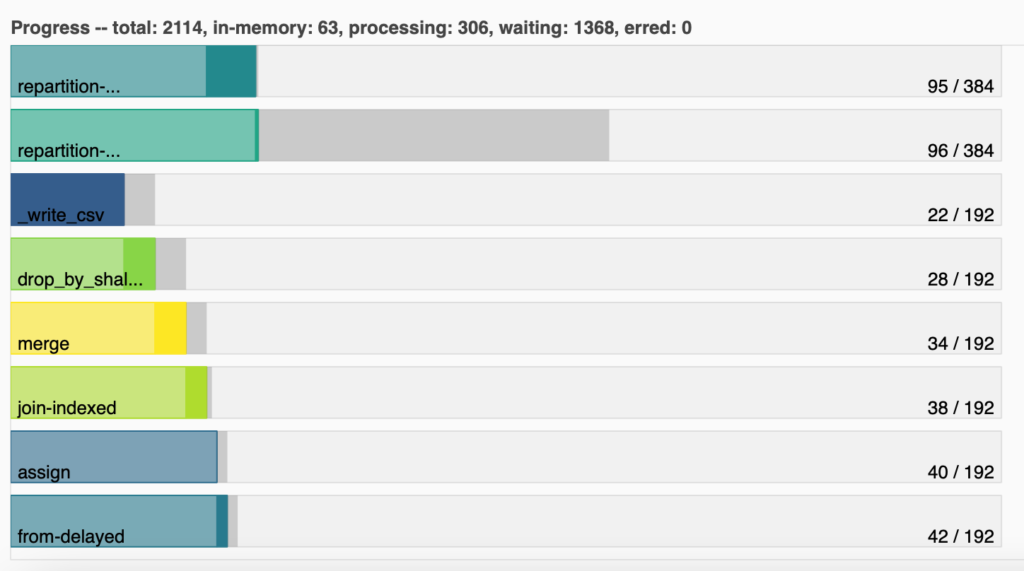
What we are seeing in here are some main computations that Dask has to do, the amount of partitions is working with (192), and how many of those partitions completed each computation. For example, we can see that _write_csv, which saves the data into a CSV and thus is the last step, has already been computed by 22 partitions, even though there are so many partitions that have not even computed anything. Know here more about Graph tasks and dask computation.

Indexing

Defining Pandas’ indexes increases performance when filtering by the index or in functions such as join.

Dask defines the data that goes into each partition by using the index. This greatly impacts the performance of the following scenarios:

1. Computations that access data in a single partition are fast. For example, having an index on a date column and selecting dates that near to each other.
2. Operations that have to look for data in other partitions are slower (Dask has to change the partition that is in RAM). From the prior example, selecting a date that is not in the current partition, or sorting and joining.
3. Looking for data without using an index forces Dask to scan all the dataframe—swapping many partitions from RAM—, being way slower: sorting and joining on columns that are not indexed.

Here you have more info.

So, the rule of thumb is: define an index on the column you are going to use when executing a costly operation like filter, sort, join, and groupby. However, try to reindex as less as possible (find a balance), as it is a very expensive operation.

The common place to define an index Dask is when reading data:

df = dd.read_sql_table(
    table,
    uri='database uri',
    index_col='ID',
    ...
)

4. Tune Dask

As you can see from subsection 3, one of the keys in Dask is how the partitions are done. Dask takes many liberties when automatically partitioning data. They work fairly well, but for big datasets you might still get Out of memory errors: this means that your partitions are so big that they still don’t fit in RAM. Our objective is, then, to tune the size of the partitions so we don’t get out of memory errors, but without ending with small partitions that would trigger Dask to constantly load and save them—with the implied overhead. Dask goes into more details in here.

The easy way of tuning this is by using the npartitions parameter of the reader functions:

df = dd.read_sql_table(
    table,
    uri='database uri',
    index_col='ID',
    npartitions=?,
    ...
)

Where ? is the magic number we want to find. The process is simple:

1. We write a big npartitions number (the bigger the number the smaller the partitions are).
2. We execute and check the dashboard (see below for examples). On the one hand, if we start to see that we are topping the RAM of our nodes and spilling data to disk often—or we get an out of memory error—we increase the number and execute again. On the other hand, if we see that there is great amount of RAM not being used, we reduce the number and execute again.

For example, for my data, I tried with three npartitions: 120, 140, and 160. For 120, I got an out of memory error. The following two graphs represent the Bytes stored graph from the dashboard for the 140 (left) and 160 (right) npartitions:

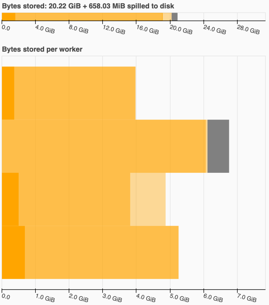
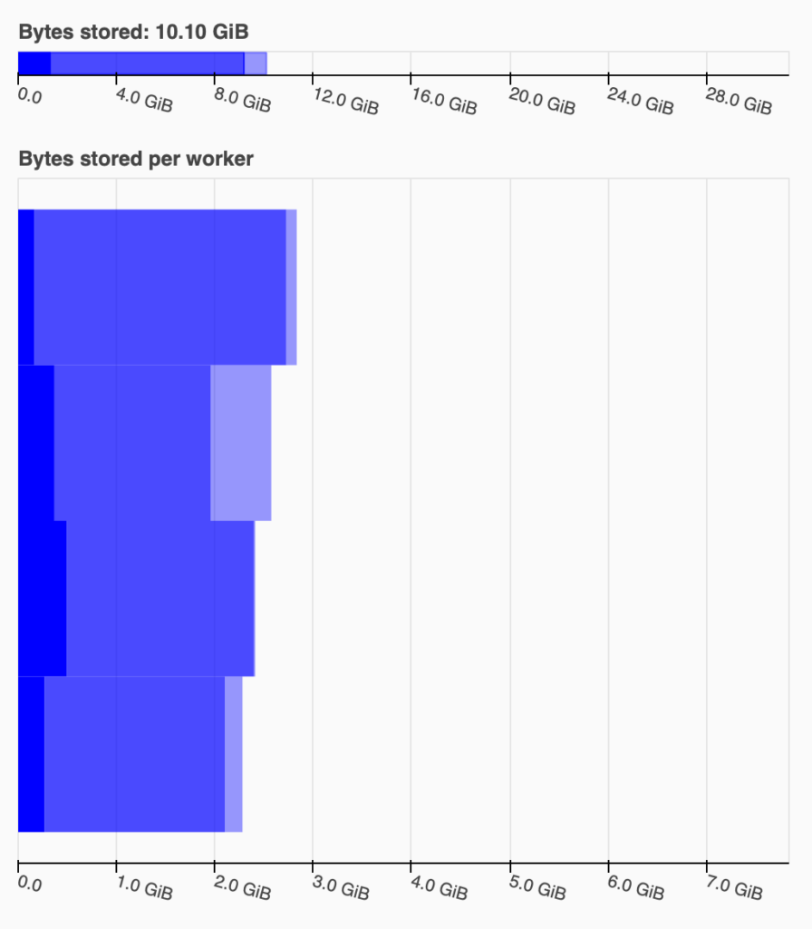
Note that I was using a PC with a 32GB of RAM for these tests. In the left graph, you can see that Dask has spilled ~658MiB into disk, meaning that is saving partitions into a temporal file. In my experience, when this happens, you are too close to an out of memory, so try to avoid it.

4.1 An example

The following is an example of what an optimized Dask execution would look like (unfortunately you cannot execute this example as it reads data from a non-existing database):

from dask.distributed import Client
import numpy as np

client = Client()
print(client.dashboard_link)
df = dd.read_sql_table(
    'meteo_data',
    uri='postgresql://user:pass@uri/meteo-db',
    index_col='Station',
    npartitions=120,
    meta=pd.DataFrame(
        {
            'Created': pd.Series([], dtype='datetime64[ns]'),
            'Created Hour': pd.Series([], dtype=str),
            'Station': pd.Series([], dtype='category'),
            'Measure': pd.Series([], dtype='category'),
            'Value': pd.Series([], dtype=np.float16)
        }
    )
)
grouped_df = df.groupby(
    [
        'Station',
        'Measure'
    ]
).agg(
    {
        'Value': np.mean
    }
)
grouped_df.to_csv('result-*.csv')

You can see how the index represents one of the columns used to group by, how we define the dtypes when reading the data, and how we finally save the resulting dataframe in a CSV.

5. Beyond multiprocessing

Dask is not only capable of multiprocessing—executing Pandas through all cores of our machine—but of clustering: executing Pandas through different interconnected computers. You can explore this option if a computer is truly not enough.

Finally, you can accelerate the computation further by using your computer’s GPU, or the high performance python compiler Numba.

Conclusion

In this post we have seen 3 ways of optimizing Pandas execution: 1. lopping correctly using vectorization and built-ins, 2. defining the most performant datatypes, and 3. parallelizing and unlocking greater-than-RAM datasets with Dask.

These are the biggest three things that worked for me, but I would love to hear yours in the comments.

Happy coding 🙂